Back-propagation Demystified [Part 3]

This is a continuation of Part 1 and Part 2 of the back-propagation demystified series. In this post I’ll be talking about computational graphs in Tensorflow.

Tensorflow uses dataflow graph to represent computation in terms of the dependencies between individual operations. This leads to a low-level programming model in which one defines the dataflow graph, then creates a TensorFlow session to run parts of the graph across a set of local and remote devices.

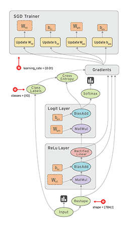
An example of a dataflow or computational graph in TensorFlow is shown below.

Computational graph example in TensorFlow (Source: Tensorflow Graph Guide)

In Tensorflow, any kind of computation is represented as an instance of tf.Graph object. These objects consist of a set of instances of tf.Tensor objects and tf.Operation objects. In Tensorflow, the tf.Tensor objects serve as edges while the tf.Operation serve as nodes which are then added to the tf.Graph instance.

In TensorFlow, a tf.Session() object stores the context under which a computation is performed. It is a class for running TensorFlow operations. A Session object encapsulates the environment in which Operation objects are executed, and Tensor objects are evaluated.

Now, let us construct the computational graph in Tensorflow using the example used in Part 1 of the post.

# Import the libraries
import tensorflow as tf
import os

#Create input placeholders for the graph variables
a = tf.placeholder(tf.float32,shape=(1,),name='a')
b = tf.placeholder(tf.float32,shape=(1,),name='b')
c = tf.placeholder(tf.float32,shape=(1,),name='c')
d = tf.placeholder(tf.float32,shape=(1,),name='d')

# Create graphs from the placeholders
u = tf.multiply(a,b,name='u')
t = tf.log(d,name='t')
v = tf.multiply(t,c,name='v')
e = tf.add(u,v,name='e')

# Run the session
with tf.Session() as sess:
    # Calculate the gradients of e and print them
    print('de/da: ',sess.run(tf.gradients(e,a),{a: [2.0],b: [3.0], c: [5.0], d: [10.0]})[0][0])
    print('de/db: ',sess.run(tf.gradients(e,b),{a: [2.0],b: [3.0], c: [5.0], d: [10.0]})[0][0])
    print('de/dc: ',sess.run(tf.gradients(e,c),{a: [2.0],b: [3.0], c: [5.0], d: [10.0]})[0][0])
    print('de/dd: ',sess.run(tf.gradients(e,d),{a: [2.0],b: [3.0], c: [5.0], d: [10.0]})[0][0])
    # Write the tensorboard object
    writer = tf.summary.FileWriter('./graphs', sess.graph)

We start by creating four placeholders. A tensorflow placeholder is a proxy for a tensor which is fed during session execution. It requires the feed_dict argument to Session.run(), Tensor.eval(), or Operation.run().

Next, we use the tensorflow operations namely add, log and multiply to construct the example computational graph from the defined placeholders.

Once the graph is constructed, next step is to run it in a Session. Python has a with statement which takes care of opening and closing the Session. In the session scope we run the tf.gradients function to obtain the required gradients for our example. The output is shown below.

TensorFlow has a utility called tensorboard gives you a pictorial representation of the computational graphs with a lot of visualization functionalities. The graph for the previous example is shown below.

As can be seen, the graph is same as the one we constructed in the example picture. The jupyter notebook can be found at: https://github.com/msminhas93/ComputationalGraphs

With this we reach the end of the “Back-propagation Demystified” series. The key takeaways are as follows.

• Back-propagation is used for calculating the gradients required for the gradient descent based optimizations for training deep learning networks.
• Calculating an analytical expression for gradients is straightforward but computational expensive.
• Computational graphs are methods of representing mathematical expressions and in the case of deep learning models, these are like a descriptive language giving the functional description of the required computations.
• Deep learning frameworks such as PyTorch and TensorFlow etc. depend on the creation of these computational graphs to implement the back-propagation algorithm for the defined networks for the calculation of gradients.

Finally, here is a comparison of how computational graphs are represented in PyTorch and Tensorlfow.

Thank you for reading. Please like, share and subscribe if you liked the post.