Gradient Descent Optimization [Part 2]

This is a continuation of Gradient Descent Optimization [Part 1]. In this post I’ll be taking examples and explaining how the choice of learning rate and the start point affects the convergence of the algorithm.

We will start with a 1D case, since it is easiest to visualize. The equation we are using is same as the one I used in this post. The equation and its derivative are given below.

I’ll show how to manually implement the code in python using numpy and matplotlib.

# Define the equation function
def loss_surface(x):
    return np.power(x,4)+ np.power(x,3) - 6*np.power(x,2)
#Define the gradient function
def parabola_grad(x):
    return 4*np.power(x,3)+3*np.power(x,2)-12*x
# Select a random start point in the axis range
x0 = np.random.uniform(-3,3)
# Specify the learning rate
lr=0.01

# Initialize a list to keep track of the gradient descent points
x_l = [x0]

#Perform gradient descent
for i in range(100):
    # Update the x0 value 
    x0=x0-parabola_grad(x0)*lr
    # Add points to the list
    x_l.append(x0)
x_l = np.array(x_l)    
y_l = loss_surface(x_l)
# Plot the curve and points
plt.plot(x,y);
plt.plot(x_l[0],y_l[0],'rx');
plt.plot(x_l[-1],y_l[-1],'kx');
plt.plot(x_l,y_l,'r-');

The graphs of various combinations of start point and learning rates are shown in following figure.

The equation under consideration has two minima. We want to find the global minimum using the gradient descent algorithm. I’ll be explaining the figures filled by row. The number of iterations is kept as 10 for all the examples. I’ve varied the learning rate and the initial start point to show you how it affects the algorithm. First five plots show that if start point and number of iterations is kept the same, larger the learning rate faster the algorithm descends. But in those cases the algorithm got stuck at a local minimum. In plot seven we see that due to the large learning rate coupled with the steep slope at the start point the algorithm took a large jump to the global minimum.

Even though large learning rates can cause faster convergence, there are chances of your algorithm moving away from the minimum because of the large effective step size. Take a look at the last figure, the starting point enabled the algorithm to go to the global minimum but the large learning rate caused the algorithm to diverge. One more case is shown in the second last figure. The point was initialized at a critical point which has a zero derivative at that point. No matter how large your learning rate or how many steps you take the algorithm won’t move from that point.

From above examples we see that learning rate has to be chosen such that it is not too low so that the gradient is over-damped or too high for the gradient to blow up the step size. The initialization of the start point is crucial can get you the global minimum or the local. The number of steps to be taken also matter.

Let us proceed with a few 2D examples.

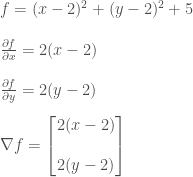
The first examples is of a paraboloid and its equation is as follows.

I’ll be using sympy for this tutorial. This allows you to do symbolic computations on equations. Even if you don’t know calculus, you can use the code to try out different equations and experiment around.

Following code creates a function f1 using the symbolic representation of sympy and calculates the partial derivatives w.r.t. x and y to calculate the gradient.

#import the libraries
from mpl_toolkits import mplot3d
%matplotlib qt
import numpy as np
import matplotlib.pyplot as plt

# Define the sympy symbols to be used in the function
x = symbols('x')
y = symbols('y')
#Define the function in terms of x and y
f1 = (x-2) ** 2 + (y-2)**2+5

# Calculate the partial derivatives of f1 w.r.t. x and y 
f1x = diff(f1,x)
f1y = diff(f1,y)

Following code implements the gradient descent. We are updating the x and y values using the appropriate gradient components.

# Define a function optimized for numpy array calculation
# in sympy 
f = lambdify([x,y],f1,'numpy')

# Define the x and y grid arrays
x_grid = np.linspace(-3, 3, 30)
y_grid = np.linspace(-3, 3, 30)
# Create mesh grid for surface plot
X, Y = np.meshgrid(x_grid,y_grid)

#Define the surface function using the lambdify function 
Z = f(X,Y)

#Select a start point
x0,y0 = (3,3)
#Initialize a list for storing the gradient descent points
xlist = [x0]
ylist = [y0]

#Specify the learning rate
lr=0.001

#Perform gradient descent
for i in range(100):
    # Update the x and y values using the negative gradient values
    x0-=f1x.evalf(subs={x:x0,y:y0})*lr
    y0-=f1y.evalf(subs={x:x0,y:y0})*lr
    # Append to the list to keep track of the points
    xlist.append(x0)
    ylist.append(y0)

xarr = np.array(xlist,dtype='float64')
yarr = np.array(ylist,dtype='float64')   
zlist = list(f(xarr,yarr))

#Plot the surface and points
ax = plt.axes(projection='3d')
ax.plot_surface(X, Y, Z, rstride=1, cstride=1,
                cmap='viridis', edgecolor='none')
# ax.plot(xlist,ylist,zlist,markerfacecolor='r', markeredgecolor='r', marker='o', markersize=10, alpha=0.6)
ax.plot(xlist,ylist,zlist,'ro',markersize=10,alpha=0.6)
ax.set_title('Gradient Descent');
ax.set_aspect('equal')

Following figure shows two views of the 3D plot.

One thing immediately evident from the plot is as the algorithm reaches near the minimum the gradient value decreases and therefore the step size decreases. As I mentioned at the start of the post, the technique remains the same for n dimensional case. The observations that we draw in lower dimensions can be almost always extended to the higher dimensional case with little or no modifications.

To give you a flavor for different surfaces, following are two more examples of 2D gradient descent. As discussed earlier the initialization matters and will ultimately decide where you end up at the end.

I’ve made a python utility that let’s you play around with the learning rate, number of iterations and initial start point to see how these affect the algorithm performance for the 1D example. The code for this as well as the 2D function plots is available at following repository.
https://github.com/msminhas93/GradientDescentTutorial

In the next post I’ll discuss few tips and tricks for gradient descent specific to deep learning applications.

If you learnt something from the post, please do like, share and subscribe.