
This is a continuation of the Gradient Descent series Part0, Part1 and Part2. So far we’ve seen the algorithm and taken 1D and 2D examples to analyse how their choice affects the convergence.
In the context of deep learning gradient descent can be classified into following categories.
- Stochastic Gradient Descent
- Mini-batch Gradient Descent
- Batch Gradient Descent
Stochastic Gradient Descent: Suppose you want to minimize an objective function that is written as a sum of differentiable functions.
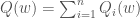
Each term 

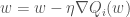
Standard gradient descent (batch gradient descent) is given as follows.

where 
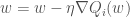
Stochastic Gradient Descent (SGD) considers only a subset of summand functions at every iteration. This can be effective for large-scale problems. The gradient of 
This update needs to be done for each training example. Several passes might be necessary over the training set until the algorithm converges.
Pseudo-code for SGD:
- Choose an initial value of
and
.
- Repeat until converged.
- Randomly shuffle data points in the training set.
- For
, do:
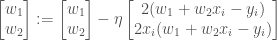
Example:
Suppose

The objective function is:

The update rule for SGD then is as follows.
Mini Batch Gradient Descent:
- Batch gradient descent uses all
data points in each iteration.
- Stochastic gradient descent uses
data point in each iteration.
- Mini-batch gradient descent uses
data points in each iteration.
Pseudo-code for Mini-Batch Gradient Descent:
- Choose an initial value of
- Choose for example
- Repeat until converged.
- Randomly shuffle data points in the training set.
- For
, do:


Few points on the three variants.
- SGD is noisier than the other two variants because it is updated per example.
- SGD is often called an online machine learning algorithm because it updates the model for each training example.
- SGD is computationally more expensive than the other variants because it per example.
- SGD is jittery and cause convergence to a minimum difficult.
- Mini-batch gradient descent allows you to take the advantage of your GPU and process multiple examples in one go therefore reducing the training time.
- Batch gradient descent is practically infeasible unless you have a small data-set which can fit into the available memory.
Choice of mini-batch size parameter #latex b$ depends on your GPU, data-set and the model. A rule of thumb is to choose a size in multiples of 8. Generally, 32 is a good number to start with. If you choose your number too high or low then the algorithm can become slower. In the former case, computations could become slower because you are putting a lot of load on the GPU. While in the latter case, lower mini-batch size underutilizes your GPU. Finding the right balance for your case is important.
Tuning the learning rate
If
A common practice is to make 
-
, where
and
are constants.
, where
is the initial learning rate and
One can use interval based learning rate schedule too. For example:

where
The first iterations cause large changes in
There is something called as cyclical learning rates where you use a periodic function for scheduling. You can read more about it here.
This wraps up the discussion for Gradient Descent and concludes the series Part0, Part1, Part2 and Part3.
To summarize:
- Gradient descent is an optimization algorithm that is used in deep learning to minimize the cost function w.r.t. the model parameters.
- It does not guarantee convergence to the global minimum.
- The convergence depends on the start point, learning rate and number of iterations.
- In practice, mini-batch gradient descent is used with a batch size value of 32 (this can vary depending on your application).

Gosh that’s confusing 😂 how do you do that?!
LikeLike
I tried to explain it in as easy language as possible though. 😀
LikeLiked by 1 person
You’re just very smart 😀 I’m not tho 😂
LikeLiked by 1 person